How and Why to Use an Anti-Aliasing Filter
Q: What is an anti-alias filter, and do I need one?
A: At its simplest an anti-alias filter removes unwanted high-frequency signals from the signals you want to measure. Let’s look at why you might need one.
When we see a signal on an analog oscilloscope, the signal goes through every voltage shown on the signal trace. That means we see a continuous signal. When we use an analog-to-digital converter (ADC) we have only a set of discrete values that give us voltages at equal time intervals. This transition from continuous signals to discrete samples can cause problems unless you understand the characteristics of signals you want to measure.
The graph below plots seven values obtained by an ADC at about 6 ksamples/sec. Can you determine with certainty the signal that provided these voltages?
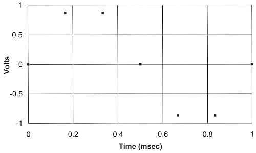
They might have come from a sine wave such as the one below that shows a continuous 1-kHz sine wave and the seven ADC samples. You might say, “OK, that’s the signal because the points fit exactly.” But you’re in for a surprise.
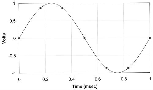
The same seven ADC measurements also can arise from a 7-kHz signal with the same amplitude, as shown below. When you examine only the seven points shown earlier, can you say for certain which signal, 1-kHz or 7-kHz, they represent? You cannot. The seven values also could come from measurements of other signals, and not necessarily sine waves.

Engineers call this effect aliasing because it’s almost as if the 7-kHz signal slipped through in disguise and took the “identity” of the 1-kHz signal. You cannot unambiguously identify the original signal based only on the seven ADC measurements. So what can we do? A bit of background information and then a solution.
In the early 1950s, Harry Nyquist (1889 1976) and Claude Shannon (1916 2001), both at Bell Laboratories, recognized the problem caused by sampling a signal. They published a theorem that explained the need to sample a real-world signal at more than two times the highest-frequency component present in a signal of interest. Today engineers refer to this relationship as the NyquistShannon sampling theorem or just the Nyquist criterion. So if you plan to measure a 1-kHz sine-wave signal with an ADC, you must sample at a rate greater than 2 ksamples/sec. And, you must remove higher-frequency signals that can “alias” to lower frequencies and distort measurements.
Q: So I need a low-pass filter to remove unwanted signals above 1 kHz. But how do I describe it to a supplier?
A: The Nyquist theorem actually says we must sample at more than twice the frequency of a signal’s bandwidth. When you have a sine wave, frequency equals bandwidth. So for the sake of simplicity I’ll use a 600-Hz sine-wave signal as an example. Assume we have a 12-bit ADC and the signal will span the entire 0- to 2.5-volt input range.
We cannot buy or make a brick-wall filter that passes a signal at 600 Hz and blocks all signals above 601 Hz. Low-pass analog filters have a characteristic slope, or roll-off, that shows how much signals get attenuated as frequency increases. And engineers usually specify a filter cut-off frequency (fc); the point at which signal attenuation becomes -3 decibels (dB). This information often appears on a Bode plot of attenuation in decibels (dB) vs. frequency (Hz).
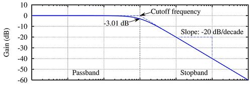
This Bode plot uses a logarithmic scale for frequency. The attenuation in decibels (dB)–shown here as a “negative gain”–already represents the logarithm of an input-output signal ratio. Courtesy of the Wikimedia Commons.
To simplify the mathematics of filter design, I recommend the free FilterLab filter-design software from Microchip Technology. It lets people examine several filter types and their characteristics based on the characteristics they need. I have used the software to create filters and the following examples come from FilterLab. For more information, visit: http://www.microchip.com/pagehandler/en_us/devtools/filterlab-filter-design-software.html. FilterLab also can produce a schematic diagram of a filter with the characteristics you select.
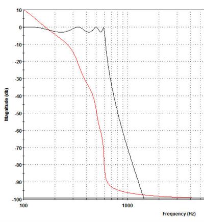
To properly filter the 600-Hz test signal before it reaches an ADC we want no attenuation at 600 Hz, and a steep attenuation of signals above that frequency. The figure below provides a FilterLab plot of attenuation vs. frequency for an 8-pole Butterworth filter with a 700-Hz cut-off. (The red line represents phase shift in the filter and I’ll ignore it in this discussion. The word “pole” refers to something called the Z transform of a filter’s impulse response. For more information, visit: http://sound.stackexchange.com/questions/24637/what-does-poles-mean-in-relation-to-a-filter.)

The next diagram shows a steeper frequency cutoff with an 8-pole Chebychev low-pass filter, but at the expense of -3 dB attenuation “ripples” at frequencies in the 0-600-Hz passband. I find a Butterworth anti-alias filter works well in most cases and it has no “ripple” in the passband.
Here is the schematic diagram for the Butterworth filter described above:

Q: The Butterworth filter gets to -100 dB at around 3000 Hz, so should I set the ADC to sample at a rate substantially above 6000 samples/sec?
A: Before you determine a sample rate, look at the resolution of the ADC used to digitize the signal. A 12-bit ADC has a resolution of 1 part in 4096, which we express in decibels with the equation:
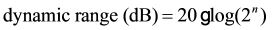
Here n equals the ADC’s number of bits. For the 12-bit ADC, we calculate a dynamic range of 72 dB. That means the ADC cannot measure signals attenuated below -72 dB. In other words, signals below -72 dB don’t exceed the voltage for ±1/2 LSB. (If you want to include a small margin, consider an attenuation of -75 dB on the plot.)
If you look at the Butterworth filter Bode plot again, you see the -72-dB point on the attenuation line occurs at about 2000 Hz. Thus the Nyquist sample rate must exceed 4000 samples/sec, so you can sample at a slower rate that you might expect at first glance. Always treat the Nyquist sample rate as a starting point. In practice I use a sample rate 5 to 10 times that specified by the Nyquist theorem.
Keep in mind that although our 8-pole Butterworth will attenuate signals at frequencies above 600 Hz, signals between that frequency and the frequency at the -72 dB point will still appear in your sampled data.
Q: My equipment doesn’t output a sine wave. Do the same filter assumptions and calculations apply?
A: They do, but your signal might include information at frequencies higher than you expect. You must take into account higher-frequency signal components and whether you need them or can do without them. A spectrum analyzer will give you a display of frequency components in a signal. A mathematical fast Fourier transform (FFT) of signals from your sensors also will show frequency components. Microsoft Excel can perform an FFT on your test data. Only you can determine which signals contribute useful information and which are just noise that could interfere with measurements.
A 1-kHz square wave provides a good example. We could not just sample at a rate of, say, 5- or 10-kHz/second because a square wave includes many higher-frequency components. Instead, we look at the bandwidth of the square wave.
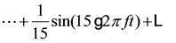
A perfect square wave–one with an instantaneous voltage change–comprises the sum of an infinite number of smaller and smaller portions of sine-wave harmonics. With enough terms to sum, the equation shown below will eventually produce a perfect square-wave plot. Here the letter f represents the fundamental frequency and t represents time:

An animation lets you see the effect of summing additional odd harmonics to create a square wave. Visit: http://en.wikibooks.org/wiki/Trigonometry/A_Square_Wave_in_Sines and scroll to the bottom of the page.
To capture all the sine-wave harmonics in a square wave would require an impossibly large bandwidth, which no ADC can provide. An Excel plot of a calculated square wave out to the 15th harmonic appears below. (Even with eight polynomial terms, we still get a “rough” square wave.)
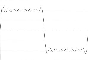
Square-wave plot from an Excel spreadsheet includes frequency components out to the 15th harmonic.
Suppose an engineer specifies the need to capture 2.5-volt square-wave signals with a 1-kHz fundamental frequency out to the 15th-harmonic frequency. That means we need samples of 15th of the amplitude at 15 times the fundamental frequency, or 15 kHz:
1. Can the given ADC–12 bits with a 2.5-volt input range–measure such a small signal? The amplitude of the 15th harmonic comes to:

The ADC can measure 611 ?volts/step (1 LSB), so the ADC will easily measure the 15th harmonic signal. In fact the ADC can measure amplitudes out to several thousand harmonics. (Thankfully, real-world square waves have finite rise and fall times and do not include that many harmonics. Also, cables, connectors, components, and circuits attenuate many of the higher-frequency harmonics as a matter of course.)
2. To remove higher-frequency harmonics before they reach the ADC you need an anti-alias filter. The filter must have a cutoff frequency such that it will not attenuate the 15th harmonic. The Microchip Technology FilterLab software calculates the response for an 8-pole Butterworth filter. I adjusted the cut-off frequency to get an attenuation of -0.1 dB at 15 kHz, and a -3 dB attenuation at 18 kHz. See the Bode plot below.

As noted earlier, a 12-bit ADC has a 72-dB dynamic range, which the filter reaches at about 54 kHz. So the sample rate must exceed 108 ksamples/sec. Given my guidelines, that means a real-world sample rate between 270 and 540 ksamples/sec. So although we started with a 1-kHz square wave, we must sample at a much greater rate. Again, a Chebychev low-pass filter offers a faster cutoff but the filter attenuates some of the signals below 15 kHz.
Most signals in process industries do not require such a high sample rate. I provide the square wave example to illustrate that what look like low-frequency signals can include high-frequency components you must take into account when you think about an anti-alias filter.